I recently got interested in second order autoregressive processes ("AR(2)" processes), after spending quite some time working only with first order ones... It was time to get an extra degree of freedom/complexity ! However, I didn't have much intuition about the behavior of these models and neither about how to "tune the knobs" that set this behavior so I spent some time on this subject.
For the sake of clarity, let's write down a definition/notation for an AR(2) process :
with the real numbers a1 and a2 being the two parameters that tune the "behavior" of the process. may be call the "input" in the context of linear filters, while "innovation" (i.e. a white noise input) would better fit in the context of random processes. A nice property of AR(2) processes, as opposed to AR(1) is their ability to capture slowly oscillating behaviors, like ocean waves. Also, within the AR(2) model, AR(1) is included as the special case a2 = 0.
Bits of a non-interactive study
In order to understand the interplay of the two parameters a1 and a2, I spent extensive time doing paper-based analytical/theoretical studies. I also created a IPython Notebook which I should publish when there is proper Notebook -> HTML conversion system (edit: now available on nbviewer). Most of the AR(2) behavior is governed by the characteristic polynomial . This polynomial helps in showing that there are two regimes : the one with two real roots (when
) and the one with two complex-conjugate roots (when
) where I can get my long-awaited slow oscillations. A third regime is the special case of a double root
which I don't think is of a special interest.
Beyond the study of the root, I also computed the variance of the process and its spectral density. I found both not so easy to compute !
Creating an interactive tool
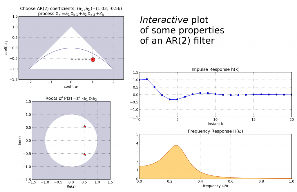
After the static paper-based study and the still semi-static computer-based study, where I was able to derive and plot the impulse response and some realization of random trajectories, I wanted to get a real-time interactive experience of the interplay of the two parameters a1 and a2. To this end I wrote a tiny Python script, based on the event handling machinery of Matplotlib. More specifically, I started from the "looking glass" example script which I altered progressively as my understanding of event handling in Matplotlib was getting better. Here is a frozen screen capture of the resulting plots:

I put the code of this script on a GitHub Gist. This code is quite crude but it should work (assuming that you have NumPy, SciPy and Matplotlib installed). I've implemented the plots of three properties of the process:
- the root locus diagram, where one can see the transition between the two real roots and the two complex-conjugate roots as the
boundary is crossed.
- the Impulse Response (output of the filter for a discrete impulse
), implemented simply using
scipy.signal.lfilter. - the Frequency Response, which I normalized using the variance of the process so that it always has unit integral. This latter property is mainly based on my own analytical derivations so that it should not be taken as a gold reference !
My feeling about interactive plotting with Matplotlib
Overall, I felt pretty at ease with the event handling machinery of Matplotlib. I feel that writing an interactive plot didn't add too many heavy lines of code compared to a regular static plot. Also, the learning curve was very smooth, since I didn't have to learn a new plotting syntax, as opposed to some of my older attempts at dynamic plotting with Traits and Chaco. Still, I feel that if I wanted to add several parameters in a small interactive GUI, Traits would be the way to go because I haven't seen a nice library of predefined widgets in Matplotlib (it's not it's purpose anyway). So I keep the Traits and Chaco packages for future iterations !